What has the Black Death got to do with global warming? You might well ask but there is a theory that links the early onset of global warming to fluctuations in human population caused by plagues. This radical idea was put forward by William Ruddiman in his book Plows, Plagues and Petroleum and has added another dimension to our understanding of the Anthropocene. Geological time is divided into eras; the current one being the Quaternary which started some 2 million years ago with the onset of the last ice age. Some have argued that we should formally recognise a new geological era called the Anthropocene – the period of human impact. Now geological periods are defined by type sections where the international geological community agree to place an imaginary Golden Spike at the precise point between the two periods. But where should one place the Golden Spike for the start of the Anthropocene? Should it be a sequence in which you can detect the residue of the first atomic tests? Should it be the first appearance of heavy metals and coal dust associated with the Industrial Revolution? Or should it be much earlier, perhaps with the first forest clearances?
Global Warming
Hot things give out shorter wavelength radiation than cold things. So the radiation from the sun is short, it heats the Earth but only a bit, which therefore re-radiates at a much longer wavelength. Different gases absorb radiation at different wavelengths. So called greenhouse gases (e.g., methane, carbon dioxide and water vapour) allow short wave radiation to pass through the atmosphere but absorb longer wave length radiation. As they absorb the radiation the atmosphere heats up and in turn radiates heat back to Earth causing it to warm. While the media is fixated on carbon dioxide it is important to recognise that other greenhouse gases have greater impact. For example, methane is four times more effective than carbon dioxide; however it has a shorter residence time in the atmosphere before being broken down.
The commonly held view is that global warming commenced with the industrial revolution and the burning of fossil fuels. But is this correct?
Early onset of global warming and delayed glaciation?
Ruddiman (2005) put forward the controversial idea that human impact on the atmosphere may have started much earlier. The argument starts with methane.
So called Milankovitch orbital radiation variation have modulated the beat of climate change during the Quaternary. In particular the 22,000 orbital precession cycle influences the amount of solar radiation received in the tropics and therefore the intensity of the summer monsoon in both Asia and Africa. The summer monsoon is all about the rapid heating of land . The enhanced summer rainfall saturates tropical wetland and enhances methane production. The link between the precession of the equinoxes and the monsoon has been demonstrated via General Circulation Models (GCMs). We can monitor the global methane content in the past by sampling the methane trapped in ice cores. As shown in Figure 1 the total methane tracks orbital variations which determine the solar radiation received by the Earth.
 Figure 1: The relationship between methane and solar radiation. From: Ruddiman (2005)
The Quaternary Ice Age consists of a series of glacials interspersed with interglacials. For approximately the last million years the interglacials have been approximately 10,000 years long and the glacials 100,000. The last glacial (end-Pleistocene) ended about 10,000 years ago. One could therefore argue that the Holocene and the current interglacial are due to end soon! In fact the glacial cycle should be imminent.
If we use a past interglacial to predict what the methane record for the current interglacial should look like something interesting arises (Fig. 2). There is a clear departure between the two records and the question is why?
Ruddiman (2005) reviewed the various sources of methane and having done so tentatively suggested that the departure was down to humans. Specifically the irrigation of paddy fields and the domestication of cattle both of which are significant methane producers. Is this evidence of the early impact of humans on our climate?

Figure 2: Solar radiation and observed methane. From: Ruddiman (2005)
Looking at the same question or carbon dioxide is much harder because the controls on atmospheric carbon dioxide are much more complex (Fig. 3). Ruddiman (2005) also see evidence for an early rise in carbon dioxide; as early as 8,000 years. He ascribes this to forest clearance and the development of widespread agriculture. The real question and the one that has been hotly debated is could so few people have such an impact on carbon dioxide. Ruddiman (2005) believes that they could have and uses such sources as the 1089 Doomsday Book to calculate the amount of forest clearance and therefore the amount of carbon dioxide that could have been produced.
 Figure 3: Observed and predicted carbon dioxide levels. From: Ruddiman (2005)
The idea remains contentious and not all authorities believe that so few people (global population was small) could have such a large and profound effect. Notwithstanding this Ruddiman (2005) went on to explore the implications of what he had found, specifically the role of these early rises in methane and carbon dioxide might have had in delaying the onset of the next glacial cycle. Using a GCM he calculated the onset point for the development of a small ice sheet in northern Canada. The implication is that the early impact on global atmosphere may have delayed this event and lead to a more stable earth climate during the last 2,000 years. Heretical it may sound but the argument runs that global warming may have been a good thing until recently leading to the climate stability that has helped global civilisation develop.

Figure 4: Schematic showing actual and predicted temperatures with the glaciation threshold clearly shown. From: Ruddiman (2005)
Ruddiman (2005) went even further; he argued that if forest clearance was the key it must have varied with fluctuations in the human population. As it rose more land was cleared and more carbon dioxide was released. As it fell, for example due to pandemics, land would have been recolonised by trees consuming carbon dioxide. As shown in Figure 4 a severe pandemic could have brought global temperatures close to the glaciation threshold.
The bullet points below gives some idea of the frequency of pandemics prior to 1500.
- 75,000–100,000 Greece 429–426 BC Plague of Athens unknown, possibly typhus
- 5 million; 30% of population in some areas Europe, Western Asia, Northern Africa 165–180 Antonine Plague unknown, symptoms similar to smallpox
- Europe 250–266 Plague of Cyprian unknown, possibly smallpox
- 25–50 million; 40% of population Europe 541–542 Plague of Justinian plague British Isles 664-668 Plague of 664 plague, British Isles 680-686
- 75–100 million; 30–60% of population Europe 1346–1350 Black Death plague
Perhaps the best evidence comes from the colonisation of the Americas which was associated with a massive pandemic of native populations exposed to the first time to European disease such as small pox. Here there is some evidence for a correlation between declining populations and both carbon dioxide and methane levels (Nevle et al., 2011). The problem here is always on of coincidence over causality however.
Notwithstanding the radical nature of Ruddiman’s (2005) hypothesis he coherently argues that humans were having a profound impact on the Earth’s climate long before the industrial revolution. While the impact of global warming on the future of our planet may be severe, the irony is that it may have actually helped stabilise climate in the past facilitating growth in human population.
Golden Spike for the Anthropocene?
There is no doubt about the fact that human activity is modifying our environment and as such there is a compelling case for the recognition of the Anthropocene. Steffens et al., (2016) provides an excellent review of some of the issues around defining the Anthropocene and what it means. Voosen (2016) also provides an interesting blog post on the subject. You might also like to check out the new scientific journal called the Anthropocene published by Elsevier. Should the Anthropocene be formally recognised by the international association that governs geological stratigraphy the key question becomes when did it start? Or to put it in geological speak where do we place the Golden Spike (Fig. 5)?
Brown et al. (2016) provide a review of the range of geomorphological impacts associated with the Anthropocene. The numerous illustrations clearly demonstrate the impact, the problem that they are all diachronous. Diachronous (Greek dia, through + Chronos time) referrers to a geological unit which looks the same but varies in age from place to place. For example, the impact of humans on a river system may vary from catchment to catchment depending on when humans started to modify the river at each location.

Figure 5: Most formally identified geological boundaries are demarcated by an imaginary spike all though some like this one is near Pueblo, Colo. (GSSP is the acronym for Global Stratotype Section and Point. Source: Brad Sageman, Northwestern University).
Some of the possible markers include (Smith and Zeder, 2013):
- 1950s artificial radionuclides widely present in sediment caused by atomic detonations (Zalesiewicz et al., 2010).
- 1750-1800 increase in methane and carbon dioxide due to industrial revolution (Crutzen, 2002).
- 2000 BC evidence of human ecosystem engineering (Certini and Scalenghe, 2011).
- 5,000-4,000 BC methane spike from increased wet rice agriculture and cattle raising (Fuller et al., 2011).
- 8,000-5,000 BC methane and carbon dioxide rise due to forest clearance and wet rice cultivation (Ruddiman, 2005).
- 11,000-9,000 emergence of human constructions and animal domestication.
- Current Pleistoecene to Holocene boundary is as 11,700 BC.
- 13,800 BC mass extinction of Quaternary megafauna potential by humans.
The debate ranges on and a flavour of it can be got from such articles as Lewis and Maslin (2015) and Monastersky (2015). One might however usefully ask does it matter?
In a geological context the answer would normally be yes; defining the start of the Jurassic is quite a big deal for stratigraphers. It allows people to organise their local outcrops within a global framework that is agreed by all geologists working on similar deposits. However, the Anthropocene is the current and there defining its boundary is less important. In a million years’ time it might matter to a future geologist to correlate events, but for now it is much more of an academic debate (Fig. 8). Papers are there to be written and reputations made – the rather base driver for a lot of scientific endeavour – so the debate is very current and generating a lot of papers. Its importance however lies not in a defined period but as an umbrella for scientific endeavour. For example, there are lot of Quaternary Scientists out there and they have a plethora of journals and academic courses dedicated to them. The Anthropocene offers the same potential framework for the interdisciplinary scientists – ecologists, geologists, and environmental scientists – all working on the impact of humans on our planet. The recent launch of a number of Anthropocene journals is perhaps the start of this movement.
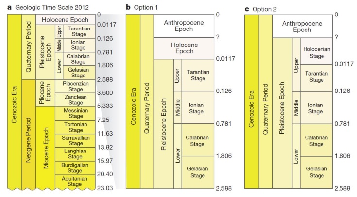 Figure 6: Different options for the Anthropocene. The left hand panel shows the current situation and on the right are the two potential options. (Source: Lewis and Maslin, 2015)
References
Brown, A.G., Tooth, S., Bullard, J.E., Thomas, D.S., Chiverrell, R.C., Plater, A.J., Murton, J., Thorndycraft, V.R., Tarolli, P., Rose, J. and Wainwright, J., 2016. The geomorphology of the Anthropocene: emergence, status and implications. Earth Surface Processes and Landforms.
Smith, B.D. and Zeder, M.A., 2013. The onset of the Anthropocene. Anthropocene, 4, pp.8-13. (Crutzen and Stoermer, 2000).
Certini, G. and Scalenghe, R., 2011. Anthropogenic soils are the golden spikes for the Anthropocene. The Holocene, p.0959683611408454.
Fuller, D.Q., Van Etten, J., Manning, K., Castillo, C., Kingwell-Banham, E., Weisskopf, A., Qin, L., Sato, Y.I. and Hijmans, R.J., 2011. The contribution of rice agriculture and livestock pastoralism to prehistoric methane levels: An archaeological assessment. The Holocene, p.0959683611398052.
Lewis and Maslin (2015) and Monastersky (2015).
Lewis, S.L., Maslin, M.A., 2015. Defining the anthropocene. Nature 519, 171-180.
Monastersky, R., 2015. Anthropocene: the human age. Nature 519, 144-147.
Nevle, R.J., Bird, D.K., Ruddiman, W.F. and Dull, R.A., 2011. Neotropical human-landscape interactions, fire, and atmospheric CO2 during European conquest. The Holocene, p.0959683611404578.
Ruddiman, W.F., 2005. Plows, Plagues, and Petroleum: How Humans Took Control of Climate. University Press
Steffen, W., Persson, Å., Deutsch, L., Zalasiewicz, J., Williams, M., Richardson, K., Crumley, C., Crutzen, P., Folke, C., Gordon, L. and Molina, M., 2011. The Anthropocene: From global change to planetary stewardship. Ambio, 40(7), pp.739-761.
Voosen, P. (2015) Geologists drive golden spike toward Anthropocene’s base http://www.eenews.net/stories/1059970036
Zalasiewicz, J., Waters, C.N., Williams, M., Barnosky, A.D., Cearreta, A., Crutzen, P., Ellis, E., Ellis, M.A., Fairchild, I.J., Grinevald, J. and Haff, P.K., 2015. When did the Anthropocene begin? A mid-twentieth century boundary level is stratigraphically optimal. Quaternary International, 383, pp.196-203.


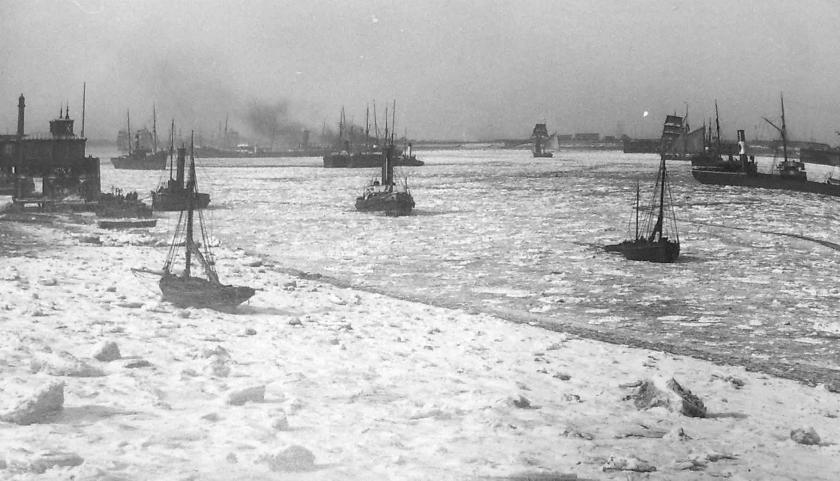 Figure 1: Photograph in 1895 of the River Thames at Gravesend.
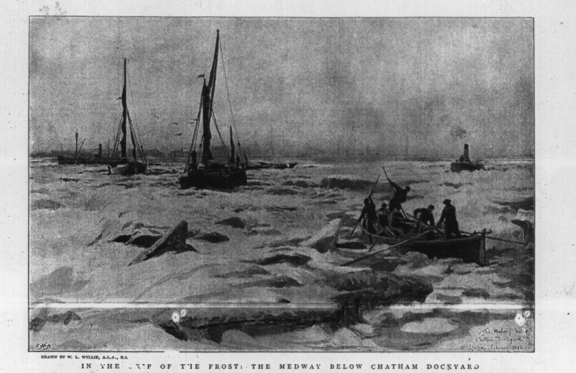


 Figure 4: Mississippi bank cross-sections organised to give a temporal model for how they evolve through time. Note the slope relaxation when the lateral undercutting from the river is removed. (Source:
 Figure 1: Reconstruction of Doggerland. (Source:
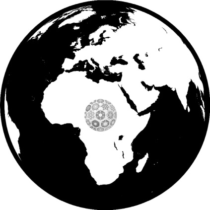


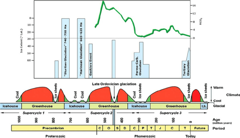 Figure 4: History of ice on Earth. Note the term ‘infra Cambrian’ was an old fashioned term used for the Neoproterozoic which is the most recent part of the Precambrian. (Source: Craig et al., 2009)
 Figure 6: Snowball Earth. (Source:


